Actor Critic Algorithms

Video link

Improving the Policy Gradient

Recall $\hat{Q}_{i,t}$ from the last lecture. $\hat{Q}_{i,t}$ is the estimate of the expected reward if you take action $\mathbf{a}_{i, t}$ in state $\mathbf{s}_{i, t}$. We can improve this estimate by replacing it with its estimate:

$$\hat{Q}_{i,t} \approx \sum_{t'=t}^T E_{\pi_\theta} \left[ r(\mathbf{s}_{t'}, \mathbf{a}_{t'}) \mid \mathbf{s}_{t}, \mathbf{a}_{t} \right]$$

If we plug this back into the reward from last lecture, we can still use the baseline function (this time adapted to be the average $\hat{Q}_{i,t}$ value $b_t = \frac{1}{N} \sum_i Q(\mathbf{s}_{i, t}, \mathbf{a}_{i, t})$) to perform better than average. The baseline depending on action leads to bias, but we can improve even further by making it depend on the state. This leads to the following function for the baseline:

$$V(\mathbf{s}_t) = E_{\mathbf{a}_t \sim \pi_\theta (\mathbf{a}_t \mid \mathbf{s}_t)} Q(\mathbf{s}_t, \mathbf{a}_t)$$

This is the average reward over all the possibilities that start in a given state--the value function! Plugging it back in we get the equation below, where $Q - V$ makes sense because it represents your estimate of how much better $\mathbf{a}_{i, t}$ is than the average action in $\mathbf{s}_{i, t}$.

$$\nabla_\theta J(\theta) \approx \frac{1}{N} \sum_{i=1}^N \sum_{t=1}^T \left[ \nabla_\theta\log \pi_\theta (\mathbf{a}_{i,t} \mid \mathbf{s}_{i,t})(Q(\mathbf{s}_{i, t}, \mathbf{a}_{i, t}) - V(\mathbf{s}_{i, t})) \right]$$

$Q - V$ is so important that it is called the Advantage function, $A$. $Q$, $V$, and $A$ are often written with the superscript $\pi$ to denote that they rely on the policy $\pi$. To recap the three:

1. $Q^\pi (\mathbf{s}_{t}, \mathbf{a}_{t})$: Total reward from taking $\mathbf{a}_{t}$ in $\mathbf{s}_{t}$
2. $V^\pi (\mathbf{s}_{t})$: Total reward from $\mathbf{s}_{t}$
3. $A^\pi (\mathbf{s}_{t}, \mathbf{a}_{t}) = Q^\pi (\mathbf{s}_{t}, \mathbf{a}_{t}) - V^\pi (\mathbf{s}_{t})$: How much better $\mathbf{a}_{t}$ is

This provides us with a large reduction in variance with the cost of a small increase in bias.

Policy Evaluation

Which of $Q^\pi$, $V^\pi$, and $A^\pi$ should we fit and what should we fit it to? We'll choose $V^\pi$ since it's only dependent on $\mathbf{s}_{t}$ and the other two functions can be approximated by it as follows:

$$\begin{align*} Q^\pi (\mathbf{s}_{t}, \mathbf{a}_{t}) &\approx r(\mathbf{s}_{t}, \mathbf{a}_{t}) + V^\pi(s_{t+1}) \\ A^\pi (\mathbf{s}_{t}, \mathbf{a}_{t}) &\approx r(\mathbf{s}_{t}, \mathbf{a}_{t}) + V^\pi(s_{t+1}) - V^\pi(s_t) \end{align*}$$

Fitting $V^\pi(s_t)$ is called policy evaluation. $J(\theta)$ can be expressed as

$$J(\theta) = E_{\mathbf{s}_{1}} \sim p(\mathbf{s}_{1}) \left[ V^\pi(\mathbf{s}_{1}) \right]$$

How can we perform policy evaluation? We can use a NN function approximator ($\phi$) for $V^\pi$ which uses the supervised regression algorithm $\mathcal{L}(\phi) = \frac{1}{2} \sum_i \left\Vert \hat{V}_\phi^\pi(\mathbf{s}_i) - y_i \right\Vert ^2$ on the training data $\left\{\left( s_{i, t}, y_{i, t} \right)\right\}$. How can we find $y_{i, t}$?

Monte Carlo Method

The Monte Carlo target estimates it using a single sample: $y_{i, t} = \sum_{t'=t}^T r(\mathbf{s}_{i, t'}, \mathbf{a}_{i, t'})$

Ideal Target

The ideal value is:

$$\begin{align} y_{i, t} &= \sum_{t'=t}^T E_{\pi_\theta} \left[ r(\mathbf{s}_{t'}, \mathbf{a}_{t'}) \mid \mathbf{s}_{i,t)} \right] \\ &\approx r(\mathbf{s}_{i, t}, \mathbf{a}_{i, t}) + V^\pi (\mathbf{s}_{i, t+1}) \\ &\approx r(\mathbf{s}_{i, t}, \mathbf{a}_{i, t}) + \hat{V}^\pi_\phi (\mathbf{s}_{i, t+1}) \end{align}$$

Note that we're directly using the previous fitted value function $\hat{V}^\pi_\phi (\mathbf{s}_{i, t+1})$, which reduces variance but slightly lowers accuracy. This is called the bootstrapped estimate.

The Algorithm

Batch Algorithm

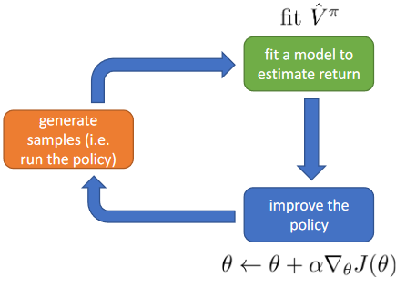
A basic batch actor-critic algorithm follows the steps below:

1. Sample $\left\{ \mathbf{s}_{i, t}, \mathbf{a}_{i, t} \right\}$ from $\pi_\theta(\mathbf{a}_{i, t} \mid \mathbf{s}_{i, t})$ (run the simulation)
2. Fit $\hat{V}_\phi^\pi(\mathbf{s})$ to the sampled reward sums
3. Evaluate $\hat{A}^\pi(\mathbf{s}_i, \mathbf{a}_i) = r(\mathbf{s}_i, \mathbf{a}_i) + \hat{V}_\phi^\pi(\mathbf{s}_i') - \hat{V}_\phi^\pi(\mathbf{s}_i)$
4. Do $\nabla_\theta J(\theta) \approx \sum_i \nabla_\theta \log \pi_\theta(\mathbf{a}_{i, t} \mid \mathbf{s}_{i, t}) \hat{A}^\pi(\mathbf{s}_{i}, \mathbf{a}_{i})$
5. Do gradient descent $\theta \leftarrow \theta + \alpha \nabla_\theta J(\theta)$

Discount Factors

If the episode length $T$ is infinite, the value function $\hat{V}_\phi^\pi$ can itself approach infinity. We can avoid this by making the agent aware of its own mortality, and having it prioritize getting rewards sooner rather than later. This is represented mathematically by a discount factor $\gamma \in [0,1]$ (usually use 0.99).

$$y_{i, t} \approx r(\mathbf{s}_{i, t}, \mathbf{a}_{i, t}) + \gamma\hat{V}^\pi_\phi (\mathbf{s}_{i, t+1})$$

When it comes to Monte Carlo policy gradients there are two options for integrating discount factors.

We can take the single-sample reward-to-go calculation and add the discount factor to it:

$$\nabla_\theta J(\theta) \approx \frac{1}{N} \sum_{i=1}^N \sum_{t=1}^T \nabla_\theta \log\pi_\theta(\mathbf{a}_{i,t} \mid \mathbf{s}_{i,t}) \left( \sum_{t'=t}^T \gamma^{t'-t} r(\mathbf{s}_{i,t'},\mathbf{a}_{i,t'}) \right)$$

We could also use the equation below, which also discounts actions in the future as well as rewards:

$$\nabla_\theta J(\theta) \approx \frac{1}{N} \sum_{i=1}^N \left( \sum_{t=1}^T \nabla_\theta \log\pi_\theta(\mathbf{a}_{i,t} \mid \mathbf{s}_{i,t}) \right) \left( \sum_{t'=t}^T \gamma^{t-1} r(\mathbf{s}_{i,t'},\mathbf{a}_{i,t'}) \right)$$

Generally we use option 1, which doesn't focus quite so much on short-term rewards.

Online Algorithm

We can also create an algorithm which updates our policy after each simulator/real-world time step, not just in batches as is the case with the standard batch algorithm:

1. Take action $\mathbf{a} \sim \pi_\theta (\mathbf{a} \mid \mathbf{s})$ to get $(\mathbf{s}, \mathbf{a}, \mathbf{s}', r)$
2. Update $\hat{V}_\phi^\pi$ using the target $r + \gamma \hat{V}_\phi^\pi(\mathbf{s'})$
3. Evaluate $\hat{A}^\pi(\mathbf{s}, \mathbf{a}) = r(\mathbf{s}, \mathbf{a}) + \hat{V}_\phi^\pi(\mathbf{s}') - \hat{V}_\phi^\pi(\mathbf{s})$
4. Find $\nabla_\theta J(\theta) \approx \nabla_\theta \log \pi_\theta(\mathbf{a} \mid \mathbf{s}) \hat{A}^\pi(\mathbf{s}, \mathbf{a})$
5. Do gradient descent $\theta \leftarrow \theta + \alpha \nabla_\theta J(\theta)$

The Architecture

A good starting point for architecture is to use two NNs: one which outputs a scalar $s \rightarrow \hat{V}_\phi^\pi(\mathbf{s})$, and the second outputs either the parameters of a continuous distribution, or the softmax of discrete actions $s \rightarrow \pi_\theta(\mathbf{a} \mid \mathbf{s})$ as the case may be. This is simple and stable, though it doesn't share features between the two networks. The other option is to use one network with a shared backbone which can output both values.

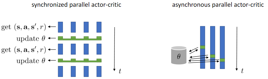
There's also the question of whether to use synchronous or asynchronous AC, when there are multiple actors.

Critics as Baselines

Actor-critic algorithms have a lower variance but are biased, whereas policy gradients have no bias, but higher variance. Critics can be used as either action- or state-dependent baselines. A method that relies on both can be referred to as a control variate.

If used as a state-dependent baseline, as shown below, we can achieve no bias with a variance very close to that of the reward.

$$\nabla_\theta J(\theta) \approx \frac{1}{N} \sum_{i=1}^N \sum_{t=1}^T \nabla_\theta \log\pi_\theta(\mathbf{a}_{i,t} \mid \mathbf{s}_{i,t}) \left( \left( \sum_{t'=t}^T \gamma^{t'-t} r(\mathbf{s}_{i,t'},\mathbf{a}_{i,t'}) \right) -\hat{V}_\phi^\pi \right)$$

If we use a control variate we get the equation below where the first term is just the policy gradient with the baseline, the second term is the gradient of the expected value under the policy of the baseline.

$$\begin{align} \nabla_\theta J(\theta) &\approx \frac{1}{N} \sum_{i=1}^N \sum_{t=1}^T \nabla_\theta \log\pi_\theta(\mathbf{a}_{i,t} \mid \mathbf{s}_{i,t}) \left( \hat{Q}_{i,t} - Q^\pi_\phi(\mathbf{s}_{i,t},\mathbf{a}_{i,t}) \right) \\ &+ \frac{1}{N} \sum_{i=1}^N \sum_{t=1}^T \nabla_\theta \mathbb{E}_{\mathbf{a}\sim \pi_\theta(\mathbf{a}_t \mid \mathbf{s}_{i,t} ) } \left[ Q^\pi_\phi (\mathbf{s}_{i,t}, \mathbf{a}_t) \right] \\ \end{align}$$

This can achieve a very low variance, with the caveat that you must be able to evaluate the second term.

Generalized Advantage Estimation

Lets compare the advantage estimator in an Actor-critic algorithm to that in a Monte Carlo algorithm. The latter has low variance, but a high bias if the value is wrong, while the former has no bias and a high variance.

$$\begin{aligned} \hat{A}_\text{C}^\pi(\mathbf{s}_t,\mathbf{a}_t) &= r(\mathbf{s}_t,\mathbf{a}_t)+\gamma\hat{V}^\pi_\phi(\mathbf{s}_{t+1})-\hat{V}^\pi_\phi(\mathbf{s}_t) \\ \hat{A}_\text{MC}^\pi(\mathbf{s}_t,\mathbf{a}_t) &= \sum_{t'=t}^\infty \gamma^{t'-t}r(\mathbf{s}_{t'},\mathbf{a}_{t'})-\hat{V}^\pi_\phi(\mathbf{s}_t) \end{aligned}$$

We'd like to combine these two to take advantages of the pros of both. This can be achieved with an n-step return estimator:

$$\hat{A}_n^\pi (\mathbf{s}_t, \mathbf{a}_t) = \sum_{t'=t}^{t+n} \gamma_{t'-t} r(\mathbf{s}_{t'}, \mathbf{a}_{t'}) - \hat{V}^\pi_\phi(\mathbf{s}_t) + \gamma^n \hat{V}^\pi_\phi(\mathbf{s}_{t+n})$$

The larger $n$ is, the lower the bias, the smaller $n$ is, the higher the variance. The first term contributes variance while the second term contributes bias. We can create a weighted average of the results of the n-step return estimators which we call Generalized Advantage Estimators (GAE) which uses the formula below where $w_n \propto \lambda^{n-1}$:

$$\begin{aligned} \hat{A}_{GAE}^\pi (\mathbf{s}_t, \mathbf{a}_t) &= \sum_{n=1}^\infty w_n \hat{A}_n^\pi (\mathbf{s}_t, \mathbf{a}_t) \\ &= \sum_{t'=t}^\infty (\gamma\lambda)^{t'=t} \left[ r(\mathbf{s}_{t'}, \mathbf{a}_{t'}) - \hat{V}^\pi_\phi(\mathbf{s}_t) + \gamma^n \hat{V}^\pi_\phi(\mathbf{s}_{t+n}) \right] \end{aligned}$$