Introduction to Deep Reinforcement Learning

Video link

Terminology

• $M = \{ S, T \}$ -- Markov chain where:
  • $S$: State space ($s \in S$)
  • $T$: Transition operator (matrix or tensor) denoting the probability of transition between states
• $M = \{ S, A, T, r \}$ -- Markov decision process where:
  • $A$: Action space ($a \in A$)
  • $r$: Reward function which is a mapping from the state and action spaces into a real number $r\: : \: S \times A \rightarrow \Re$
• $M= \{ S, A, O, T, E, r \}$ -- Partially observed Markov decision process where:
  • $O$: Observation space space ($o \in O$)
  • $E$: Emission (or observation) probability $p(o_t\mid s_t)$

Objective

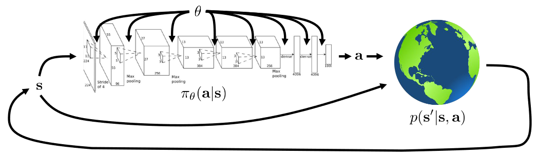
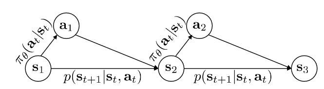
When looking at the system above, we can write down a probability distribution over trajectories, where trajectories are sequences of paired actions and states (e.g. $(s_1, a_1)$, $(s_2, a_2)$ and so on).

$$\begin{split} p_\theta(s_1, a_1, \dots, s_T, a_T) &= p(s_1) \prod^T_{t=1} \pi_\theta(a_t \mid s_t)p(s_{t+1} \mid s_t,a_t) \\ p_\theta(s_1, a_1, \dots, s_T, a_T) &= p_\theta(\tau) \\ \end{split}$$

Remember that $\pi_\theta(a_t \mid s_t)$ is the probability of an action, and $p(s_{t+1} \mid s_t,a_t)$ is the probability of a state transition.

Now we can define an objective for reinforcement learning as an expected value_under_ the trajectory distribution:

$$\theta^* = argmax_\theta E_{\tau \sim p_\theta(\tau)} \left[ \sum_t r(s_t, a_t) \right]$$

We want to maximize the expected value of the sum of rewards over the trajectory. If we augment the Markov chain by bundling states and actions so that $p((s_{t+1}, a_{t+1}\mid(s_t,a_t)) = p(s_{t+1}\mid s_t,a_t)\pi_\theta(a_{t+1}\mid s_{t+1})$ we can use the linearity of expectation to rewrite the objective such that:

$$\theta^* = argmax_\theta \sum_{t=1}^T E_{(s_t,a_t) \sim p_\theta(s_t,a_t)} \left[ r(s_t, a_t) \right]$$

Which we can use to find out what happens when $T=\infty$.

Does $p(s_t,a_t)$ converge to a single distribution as $k\rightarrow \infty$? If we assume aperiodicity and ergodicity we can write $\mu = \mathcal{T}\mu$, where $\mu$ is a stationary distribution. It follows that $(\mathcal{T}-\mathbf{I})\mu = 0$ so $\mu$ is an eigenvector of $\mathcal{T}$ with an eigenvalue of $1$. As $T \rightarrow \infty$ the sum of the expectations of the marginals becomes dominated by the stationary distribution. We can divide the expectation by $T$ to find the average:

$$\theta^* = \textrm{argmax}_\theta \frac{1}{T} \sum_{t=1}^T E_{(s_t,a_t) \sim p_\theta(s_t,a_t)} \left[ r(s_t, a_t) \right]$$

Then take the limit as $T \rightarrow \infty$ we get the expected value of the reward under the stationary distribution, where the stationary distribution $\mu = p_\theta(s,a)$:

$$\theta^* = E_{(s,a) \sim p_\theta(s,a)} \left[ r(s_t, a_t) \right]$$

Expected values can be continuous in the parameters of corresponding distributions even when the function that we're taking the expectation of is discontinuous. If we have a discontinuous reward function $r(x)$, we could have a probability distribution over some action $\pi_\theta(a)=\theta$ which is a Bernoulli random variable with parameter $\theta$. The expected value of the reward, $E_{\pi_\theta} \left[ r(x) \right]$, is actually smooth in $\theta$! The takeaway is that expected values of non-smooth and non-differentiable functions under differentiable and smooth probability distributions, are themselves smooth and differentiable.

Algorithms

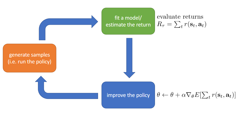
Reinforcement Learning algorithms all generally have the same three part structure:

1. Generate Samples: Run the policy in the environment, have it interact with your Markov Decision Process, and collect samples (sampled trajectories from the policy-defined trajectory distribution (i.e. run your policy in the environment)).
2. Fit Your Model: Estimate how well your policy is doing.
3. Improve Your Policy: Make your policy better given the metric calculated in step 2.

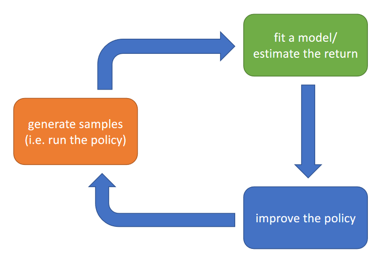
Regarding the costs of these steps:

1. Generate Samples: Depends greatly on the system in question. Real systems generate samples in real time, simulated systems can often run many times faster than real time
2. Fit Your Model: Also depends on the system! If you're doing a sum of rewards (as you would with a Policy Gradient Algorithm) it can be very fast. If you're fitting an entire neural net (as you would with reinforcement learning with back-propagation), it can be expensive.
3. Improve Your Policy: Same as 2.

Q and Value Functions

The Q Function

To recap: a reinforcement learning objective is often an expectation, defined as a sum over time for every state-action marginal. Recall that given a joint distribution of two discrete random variables $X$ and $Y$, the marginal distribution of $X$ is the probability distribution of $X$ without taking into account $Y$. The expectation can be written as:

$$E_{\tau \sim p_\theta(\tau)} \left[ \sum_{t=1}^T r(s_t, a_t) \right]$$

We can write this out recursively as a series of nested expectations, expanding it into this monster:

$$E_{s_1 \sim p(s_1)} \left[ E_{a_1 \sim \pi(a_1 \mid s_1)} \left[ r(s_1, a_1) + E_{s_2 \sim p(s_2 \mid s_1, a1)} \left[ E_{a_2 \sim \pi(a_2 \mid s_2)} \left[ r(s_2, a_2) + \dots \mid s_2 \right] \mid s_1, a_1 \right] \mid s1 \right] \right]$$

Why on earth would anyone do this? Well, what if we knew what went inside the second expectation, defined by some function called $Q$?

$$Q(s_1, a_1) = r(s_1, a_1) + E_{s_2 \sim p(s_2 \mid s_1, a1)} \left[ E_{a_2 \sim \pi(a_2 \mid s_2)} \left[ r(s_2, a_2) + \dots \mid s_2 \right] \mid s_1, a_1 \right]$$

That monstrous expansion from above becomes

$$E_{\tau \sim p_\theta(\tau)} \left[ \sum_{t=1}^T r(s_t, a_t) \right] = E_{s_1 \sim p(s_1)} \left[ E_{a_1 \sim \pi(a_1 \mid s_1)} \left[ Q(s_1, a_1) \mid s1 \right] \right]$$

If we know this $Q$ function then optimizing the policy $\pi(a_1 \mid s_1)$ at $t=1$ is easy, we can just maximize the value of $Q$. A more formal definition of the $Q$ function is:

$$Q^\pi(s_t,a_t) = \sum_{t'=t}^T E_{\pi_\theta} \left[ r(s_{t'}, a_{t'})\mid s_t, a_t \right]$$

This means that you will get the expected sum of rewards if you roll out your policy from $s_t, a_t$.

The Value Function

Defined below, the value function is essentially the same, except it's conditional only on the state, rather than the state and the action:

$$V^\pi(s_t) = \sum_{t'=t}^T E_{\pi_\theta} \left[ r(s_{t'}, a_{t'})\mid s_t \right]$$

This means that the equation below is the entirety of the reinforcement learning objective!

$$E_{s_1\sim p(s_1)} = \left[ V^\pi(s_t) \right]$$

Using Q and Value Functions

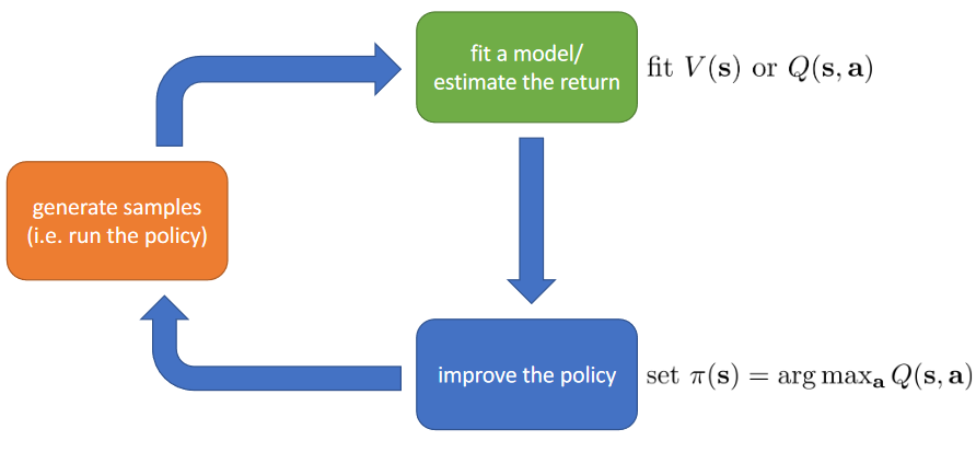
• If we have a policy $\pi$ and we know $Q^\pi(s,a)$ then we can improve $\pi$ by setting $\pi'(a\mid s)=1$ if $a=argmax_a Q^\pi(s, a)$. This means that regardless of what $\pi$ is, $\pi'$ is at least as good, and is probably better.
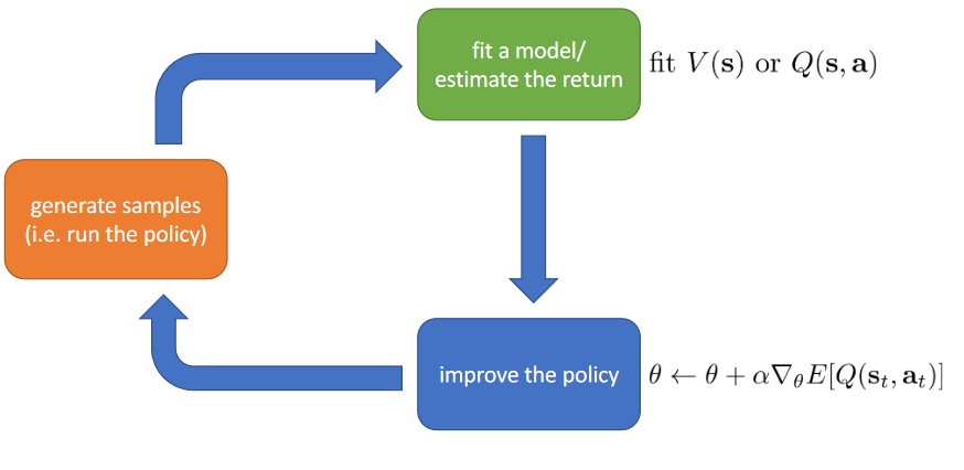
• We could also compute the gradient to increase the probability of good actions $a$ given that, if $Q^\pi(s,a) > V^\pi(s)$, then $a$ is better than average. We would do this by modifying $\pi(a\mid s)$ to increase the probability of $a$ if $Q^\pi(s,a) > V^\pi(s)$.

Types of RL Algorithms

Policy Gradient

Directly differentiate the objective w.r.t. the policy

Model Based

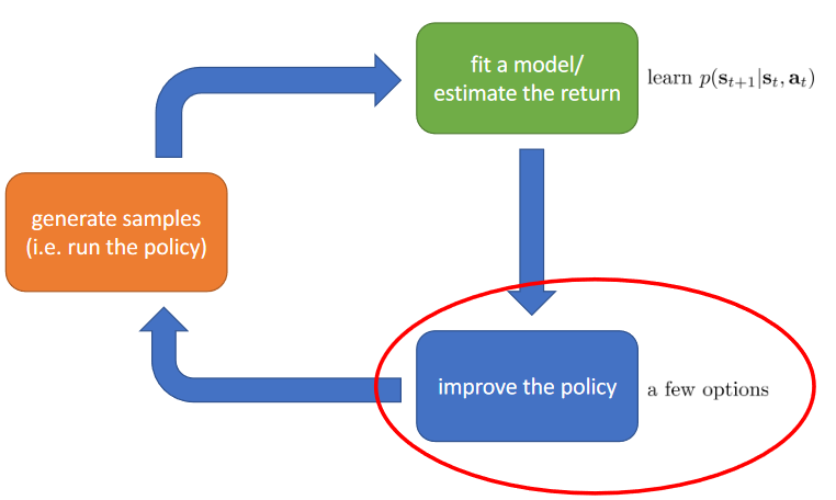
After estimating the transition model $p$ there are several options for improving the policy:

• Use the model to plan without a policy
  • Trajectory optimization; essentially backpropagation to optimize over actions (mainly continuous)
  • Discrete planning in discrete action spaces e.g. Monte Carlo tree search
• Backpropagation: use the learned model to calculate derivatives of the reward function w.r.t. the policy.
  • Can be tricky with regards to numerical stability
• Use the model to learn a Value or Q function, then use the learned function to improve the policy.

Value Function Based

$V(s)$ and $Q(s, a)$ are often NNs

Actor-critic

Improve the policy by estimating the value- or $Q$ function.

How to decide?

Some things to consider when choosing an algorithm are:

• Trade-offs:
  • Sample efficiency (how many samples do we need for a good policy?)
    • Is the algorithm on or off policy (can we improve the policy without having to regenerate samples)?
    • Real-world time $\neq$ efficiency
  • Stability and ease of use
    • Convergence criteria
    • Supervised learning is almost always gradient descent
    • Reinforcement learning is often not gradient descent
• Required assumptions:
  • Is the system fully observable? (Mitigated by adding recurrence)
  • Episodic or per-step learning?
  • Continuity or smoothness

Model comparison

Here's how each of the first three aforementioned model types compare (oversimplified):

	Policy Gradient	Model Based	Value Function
Sample Efficiency	Least efficient	Most efficient	Quite efficient
Gradient Descent?	Yes	No	No (fixed-point iteration)
Assumptions	Episodic Learning	Continuity	Full Observability and Continuity

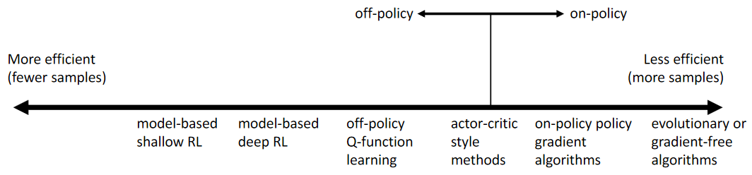
Here's how they line up on the efficiency scale: