Policy Gradients

Video link

The REINFORCE Algorithm

Given the finite-horizon case of the RL objective:

$$\theta^* = \textrm{argmax}_\theta \sum_{t=1}^T E_{(s_t,a_t) \sim p_\theta(s_t,a_t)} \left[ r(s_t, a_t) \right]$$

We can rewrite the expectation as:

$$J(\theta) = E_{(s_t,a_t) \sim p_\theta(s_t,a_t)} \left[ r(s_t, a_t) \right] \approx \frac{1}{N}\sum_i\sum_tr(s_{i,t},a_{i_t})$$

This can be approximated by making rollouts of our policy, running the policy $N$ times to collect $N$-sampled trajectories resulting in the approximation above. A bigger $N$ yields a more accurate estimation of the expected value. Now, we don't just want to estimate the objective, we actually want to improve it, by estimating it's derivative.

Note: $\sum_{t=1}^T r(s_{i,t},a_{i_t})$ will be simplified as $r(\tau)$ from here on out. {: .notice--info}

If continuous, we can expand the expectation out to the integral (sum, if discrete) of the products of the probability and the value:

$$J(\theta) = E_{\tau \sim p_\theta(\tau)} \left[ r(\tau) \right] = \int p_\theta(\tau)r(\tau)d\tau$$

The gradient of which is:

$$\nabla_\theta J(\theta) = \int\nabla_\theta p_\theta(\tau)r(\tau)d\tau$$

Note: The following identity is useful at several points in this lecture $x\nabla_\theta log x = x \frac{\nabla_\theta x}{x}$. {: .notice--info}

The identity above can be used to simplify the above equation to:

$$\nabla_\theta J(\theta) \approx \frac{1}{N} \sum_{i=1}^N \left[ \left( \sum_{i=1}^T \nabla_\theta \log\pi_\theta(a_t \mid s_t) \right) \left( \sum_{i=1}^T r(a_t, s_t) \right) \right]$$

Recall the maximum likelihood equation used in supervised learning:

$$\nabla_{\theta} J_{\mathrm{ML}}(\theta) \approx \frac{1}{N} \sum_{i=1}^{N}\left(\sum_{t=1}^{T} \nabla_{\theta} \log \pi_{\theta}\left(\mathbf{a}_{i, t} | \mathbf{s}_{i, t}\right)\right)$$

Our equation for the gradient is a reward-weighted maximum likelihood objective!

Thus, we come to the REINFORCE algorithm:

1. Sample $\{\tau^i\}$ from $\pi_\theta(\mathbf{a}_t \mid \mathbf{s}_t)$ (run the policy).
2. Use the simplified equation above to approximate $\nabla_\theta J(\theta)$.
3. Take a step of gradient descent $\theta\leftarrow\theta+\alpha\nabla_\theta J(\theta)$.

This algorithm does not require the initial state distribution or the transition probabilities. {: .notice--warning}

This algorithm does not actually use the Markov property, so it can be used in partially observed MDPs. {: .notice--warning}

Reducing Variance

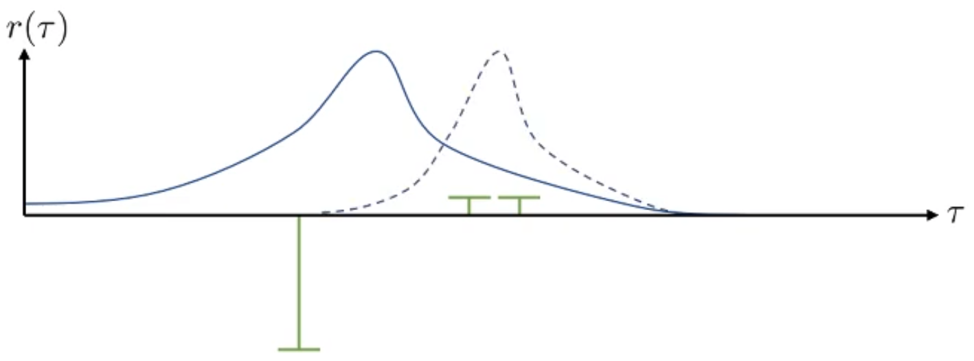
The main problem with policy gradient methods is high variance. In the image below where rewards are denoted with green lines we would expect to see the reward function move from the blue line to the blue dotted line.

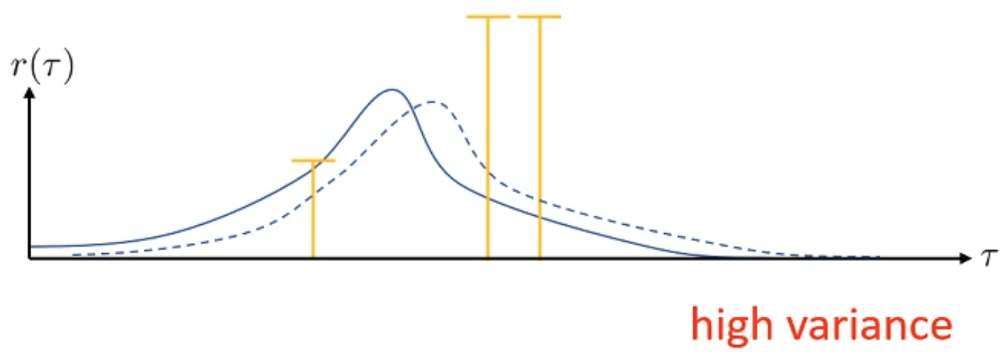
If we added an offset to the rewards we would expect the behavior below:

We can use the concept of causality to reduce the variance of the policy gradient. Causality is the idea that the policy at time $t'$ cannot affect the reward at time $t$ when $t < t'$. This allows us to simplify the equation for $\nabla_\theta J(\theta)$ to:

$$\nabla_{\theta} J(\theta) \approx \frac{1}{N} \sum_{i=1}^{N} \sum_{t=1}^{T} \nabla_{\theta} \log \pi_{\theta}(\mathbf{a}_{i, t} | \mathbf{s}_{i, t}) \hat{Q}_{i,t}$$

Where $\hat{Q}_{i,t}$ is called the "reward to go":

$$\hat{Q}_{i,t} = \sum_{t'=t}^{T} \nabla_{\theta} \log \pi_{\theta}\left(\mathbf{a}_{i, t} | \mathbf{s}_{i, t}\right)$$

Baselines

We want to center rewards around $0$, and to do so we'll subtract a quantity $b$ from them:

$$\nabla_{\theta} J(\theta) \approx \frac{1}{N} \sum_{i=1}^{N} \nabla_{\theta} \log p_{\theta}(\tau)[r(\tau) - b]$$

Where $b$ is the average reward:

$$b = \frac{1}{N} \sum_{i=1}^{N} r(\tau)$$

Subtracting this baseline does not bias the expectation. The average reward, though good, is not actually the best baseline. The best baseline is the expected reward, weighted by magnitude values:

$$b* = \frac{E[(\nabla_{\theta} \log p_{\theta}(\tau))^2r(\tau)]}{E[(\nabla_{\theta} \log p_{\theta}(\tau))^2]}$$

On/Off Policy

Policy gradients are considered to be on policy (the policy cannot be improved without having to regenerate samples). This is problematic because NNs are nonlinear and thus require taking many small steps, at each of which the samples have to be regenerated by re-running the policy. This is why policy gradient algorithms are generally good when generating samples is cheap.

Importance Sampling

We're calculating the expectation below:

$$J(\theta) = E_{\tau \sim p_\theta(\tau)} \left[r(\tau)\right]$$

But what if instead of sampling from $p_\theta(\tau)$ we had samples from another distribution, $\bar{p}_\theta(\tau)$?

Importance sampling allows us to calculate an expectation under one distribution using samples from another:

$$\begin{align} E_{x \sim p(x)} \left[f(x)\right] &= \int p(x)f(x)dx \\ &= \int \frac{q(x)}{q(x)} p(x)f(x)dx \\ &= \int q(x)\frac{p(x)}{q(x)} f(x)dx \\ &= E_{x \sim q(x)} \left[ \frac{p(x)}{q(x)} f(x) \right] \\ \end{align}$$

We can then use that $\log$ identity from HW1 to estimate the value of new parameters $\theta'$:

$$J(\theta') = E_{\tau \sim p_\theta(\tau)} \left[ \frac{p_{\theta'}(\tau)}{p_{\theta}(\tau)} r(\tau) \right]$$

The gradient of which is:

$$\nabla_{\theta'}J(\theta') = E_{\tau \sim p_\theta(\tau)} \left[ \left( \prod_{t=1}^T \frac{\pi_{\theta'}(\mathbf{a}_t \mid \mathbf{s}_t)}{\pi_{\theta}(\mathbf{a}_t \mid \mathbf{s}_t)} \right) \left( \sum_{t=1}^T \nabla_{\theta'} \log\pi_{\theta'}(\mathbf{a}_t \mid \mathbf{s}_t) \right) \left( \sum_{t=1}^T r(\mathbf{a}_t, \mathbf{s}_t) \right) \right]$$

Where the terms in parentheses are:

1. Importance weights over all timesteps (the ratio of the products of the policy probabilities).
2. Sum over all timesteps of the gradient.
3. Sum over all timesteps of the reward.

The importance weights are problematic because they're all $<1$ and thus are exponential in T, making the variance exponential as well. This kills the gradient. However, we can rewrite $J(\theta')$ as the expectation under the state action marginals to get a reasonable approximation:

$$\tilde{J(\theta)} \approx \sum_{t=1}^TE_{\mathbf{s}_t\sim p_\theta(\mathbf{s}_t)} \left[ E_{\mathbf{a}_t\sim\pi_\theta(\mathbf{a}_t|\mathbf{s}_t)} \left( \frac{\pi_{\theta}(\mathbf{a}_t|\mathbf{s}_t)}{\pi_{\theta}(\mathbf{a}_t|\mathbf{s}_t)}r(\mathbf{s}_t,\mathbf{a}_t) \right) \right]$$

Tips:

• Using large batches can reduce variance
• Tweaking learning rates is hard
• Using adaptive step sizes (e.g. with ADAM) can work

Part 6 of this lecture, Advanced Policy Gradients is not covered here. {: .notice--danger}