Supervised Learning

Video Link

Terminology

• $t$ -- Time step
• $s_t$ -- State of the system at a given time
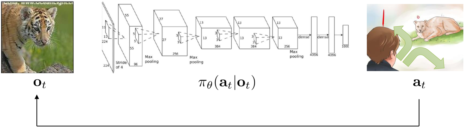
• $o_t$ -- Observation resulting from the state. Not necessarily the true state (e.g. cheetah and gazelle and car)
• $a_t$ -- Action (often a distribution)l
• $\pi_\theta(a_t \mid o_t)$ -- Policy based on $o_t$ (or $s_t$) which outputs a distribution over $a_t$ given $o_t$ ($a_t \mid o_t$)
• $\theta$ -- Policy parameters e.g. in a NN, $\theta$ = weights
• Markov Property -- Given a state, one can figure out the distribution over the next state without knowing the previous state. Given $s_t$ we can find $p(s_{t+1} \mid s_t, a_t)$ without $s_{t-1}$. It is worth noting that observations do not necessarily have the Markov Property.

Behavior Cloning

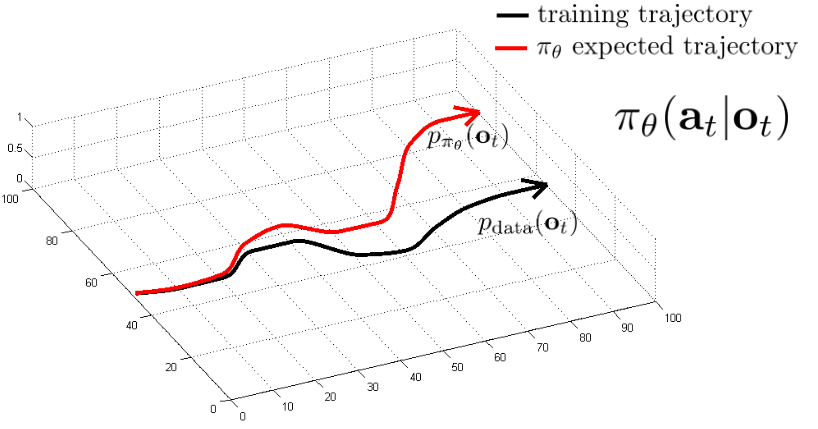
• $p_{data}(o_t)$ -- The distribution of observations seen in the training data

Often doesn't work because small errors in the learned model compound and it doesn't know how to recover (e.g. NVIDIA car). The mathematical explanation is that when running the expected trajectory we're sampling from the distribution $\pi_\theta(a_t \mid o_t)$, which was trained on the data distribution $p_{data}(o_t)$. When errors compound $p_{data}(o_t) \neq p_{\pi_\theta}(o_t)$.

Data Aggregation (DAgger)

We need $p_{\pi_\theta}(o_t) = p_{data}(o_t)$ to minimize the errors seen in behavior cloning. What if, instead of optimizing $p_{\pi_\theta}(o_t)$, we optimized $p_{data}(o_t)$? We want to collect training date from $p_{\pi_\theta}(o_t)$ instead of $p_{data}(o_t)$, which we can do by running $\pi_\theta(a_t \mid o_t)$ once we have $a_t$.

1. Train $\pi_\theta(a_t \mid o_t)$ on data from a human $D = \{ o_1, a_1, \dots, o_N, a_N \}$
2. Run $\pi_\theta(a_t \mid o_t)$ to get dataset $D_\pi = \{ o_1,\dots, o_M\}$
3. Get human to label $D_\pi$ with optimal actions $a_t$
4. Merge the two datasets $D \leftarrow D \cup D_\pi$
5. Start again from 1. with new $D$

The problematic step here is 3.

It's possible to make a model without the distributional drift problem, but first: why might we fail to fit the expert?

1. Even if $o_t$ is Markovian ($\pi_\theta(a_t \mid o_t)$), the expert (the human) might exhibit non-Markovian behavior ($\pi_\theta(a_t \mid o_1,\dots, o_t)$). This can be solved by using a recurrent neural network (RNN) with Long Short-Term Memory (LSTM).
2. The demonstrator might inconsistently choose between different modes in the distribution, which is hard to imitate. The average of two good actions could be a bad action! This can be solved with three techniques:
   1. We could represent the distribution as a mixture of Gaussians $\pi(a \mid 0)=\sum_iw_iN(\mu_i,\Sigma_i)$. This can get complicated quickly as you add more mixture elements.
   2. We could input a latent variable $\xi \simeq N(0,I)$ into the model alongside our images, essentially injecting random noise. Can theoretically represent any distribution, but can be hard to train.
   3. Autoregressive discretization is a happy medium between the two options listed above. It takes advantage of the fact that discrete actions are easily representable by a softmax distribution, sidestepping the multi-modality problem.

Cost Functions

How can we "score" actions mathematically? Cost/reward functions! If we wanted to minimize cost (note that the cost is the negative of the reward) (we do), we would minimize the expectation under a distribution over sequences of states and actions of the sum of the cost function.

$$min_\theta \ (E_{s_{1:T},a_{1:T}} \left[ \sum_t c(s_{t},a_{t}) \right])$$

A reasonable reward function could be the log probability of an expert's action:

$$r(s,a) = \log p(a = \pi^* (s) \mid s)$$

$\pi^*$ is the unknown expert policy. Another cost function could be a 0-1 loss function, which assigns a 0 if we perfectly match the expert's actions and a 1 in every other case (harsh!):

$$c(s,a) = \begin{cases} 0 \;\textrm{if}\; a = \pi^*(s) \\ 1 \;\textrm{otherwise} \\ \end{cases}$$

If we assume that $\pi_\theta(a\neq\pi^*(s)\mid s)\leq\epsilon$ for all $s\in D_{train}$ (remember the tightrope walker scenario) then the probability function is:

$$p_\theta(s_t) = (1-\epsilon)^t p_{train}(s_t)+(1-(1-\epsilon)^t)p_{mistake}(s_t)$$

Note that this is naively assuming that for all states in the training set, the probability of making a mistake at those steps is $\leq\epsilon$, where $\epsilon$ is a small number. Using the identity $(1-\epsilon)^t\geq1-\epsilon t$ for $\epsilon\in [0,1]$ we can simplify:

$$\begin{split} \mid p_\theta(s_t) - p_{train}(s_t)\mid &= (1 - (1 - \epsilon)^t)\mid p_{mistake}(s_t) - p_{train}(s_t)\mid \\ &\leq 2(1 - (1 - \epsilon)^t) \\ &\leq 2 \epsilon t \end{split}$$

The cost then becomes:

$$\begin{split} \sum_t E_{p_\theta(s_t)}[c_t] &= \sum_t \sum_{s_t} p_\theta(s_t)c_t(s_t) \\ &\leq \sum_t \sum_{s_t} \left[ p_{train}(s_t)c_t(s_t) + \mid p_\theta(s_t) - p_{train}(s_t)\mid c_{max} \right] \\ &\leq \sum_t(\epsilon + 2 \epsilon t ) \\ &\leq \epsilon T + 2 \epsilon T^2 \end{split}$$

Which is $O(\epsilon T^2)$, whereas the expectation with DAgger, $p_{train}(s) \rightarrow p_\theta(s)$, is $O(T)$.